This post is contributed by Gourav Singh Bais, who has written an excellent tutorial that shows how to build an application that uses time series data to forecast trends and events using Tensorflow and QuestDB. Thanks for the submission!

Machine Learning for Timeseries Forecasting

Machine learning is taking the world by storm, performing many tasks with human-like accuracy. In the medical field, there are now smart assistants that can check your health over time. In finance, there are tools that can predict the return on your investment with a reasonable degree of accuracy. In online marketing, there are product recommenders that suggest specific products and brands based on your purchase history.

In each of these fields, a different type of data can be used to train machine learning models. Among them, time series data is used for training machine learning algorithms where time is the crucial component.

Time series data is complex and involves time-dependent features that go beyond the scope of what traditional machine learning algorithms like Regression, Classification, and Clustering are useful for. Thankfully, there are machine learning models we can use for time series forecasting. Predictions resulted from time series forecasting may not be wholly precise due to the variable nature of time, but they do provide reasonable approximations that are applicable in a variety of fields. Let’s consider a few use cases:

• Predictive maintenance: nowadays, IoT (internet of things), AI (artificial intelligence), and integrated systems are being embedded into electronic, mechanical, and other types of devices to make them smart. These IoT devices have sensors to keep track of relevant values over time; and artificial intelligence, of which time series forecasting is a component, is used to analyze this data and make predictions regarding the approximate time at which devices may need maintenance.

• Anomaly detection: the process of detecting the rare events and observations in the functionality of systems. Identifying these events can be rather challenging, but time series forecasting helps by providing smart elements that can monitor things continuously. Cyber security, health monitoring, and fraud detection in FinTech are a few examples of systems that make use of time series analysis for anomaly detection.

• IoT data: internet of things is now becoming a concrete pillar of our economy. IoT devices have the ability to store data on a timely basis and communicate it across other devices for analysis and forecasting. One example of this is temperature prediction, in which different IoT devices are used to regularly store temperature data, while forecasting is then used to make weather-related predictions and decisions.

• Autoscaling decisions: With time series forecasting, businesses can better monitor the demand for their products or solutions over time and anticipate future demand in time to scale their services accordingly.

• Trading: Every day when the stock market opens and closes, entries are made for fluctuations in seconds. A variety of databases and file storage systems are used to store all of this information, and different time series forecasting algorithms can then be used to make price forecasts for the upcoming day, week, or even month.

In this article, we will build and train a simple machine learning model that uses time series data to forecast trends and events using TensorFlow and QuestDB.

TensorFlow and QuestDB

Time series forecasting can be carried out in different ways, including using various of machine learning algorithms like ARIMA, ETS, Simple Exponential Smoothing, and Recurrent Neural Network (RNN). The RNN is a deep learning method with multiple variations itself such as LSTM and GRU. These RNNs have feedback loops between the layers of the neural network. This makes them ideal choices for timeseries forecasting as the network can ‘remember’ for previous data. The implementation of these deep learning algorithms is made easier with the use of Google’s TensorFlow library, which supports all kinds of neural networks and deep learning algorithms.

The heart of any algorithm is the data, and that’s no different for time series forecasting. Time Series Databases (TSDBs) provide a lot more features for storing and analyzing time series data as compared to traditional databases. For this tutorial, my choice of TSDBs is QuestDB, an open source time series database with a focus on fast performance and ease of use.

Implementing Predictive Data Analysis

Now that you have a deeper awareness of time series data and time series analysis, let’s dive into a practical implementation by building an application to use this data for forecasting trends. This tutorial will use the historical exchange rate of USD to the INR data set, which you can download here in Excel format. Make sure you select the time span between 1999-2022. This data set contains three columns:

1. Date: time component that represents date of exchange rate.
2. USD: price of USD in USD (constant 1.0).
3. INR: price of USD in INR on the specific date.

As you have read, there are many different options for time series forecasting (e.g., ARIMA, ETS, Simple Exponential Smoothing, RNNs, LSTMs, GRUs, etc.). This article will focus on the deep learning solution—using neural networks to accomplish time series forecasting. Using RNNs for a small amount of data can cause an issue called vanishing gradient. Because of this reason, LSTMs and GRUs were introduced. Due to its architectural simplicity, GRU is the best option for the small amount of data you’ll be using in this tutorial.

Let’s get started!

Installing TensorFlow

TensorFlow can be easily installed with a Python package manager (PIP). Be sure to use Python 3.6 for best compatibility with TensorFlow 1.15 (as well as later versions). If you have Anaconda installed in your system, you can use the Anaconda prompt. For normal Python installation, you can use the default command prompt and write the following command to install TensorFlow:

pip install tensorflow

Note: If you are using MacOs and get a pip error, try running instead pip install tensorflow-macos

Now we need to install a few dependencies, unless you already have them locally:

pip install jupyter pandas numpy scikit-learn matplotlib openpyxl

Installing QuestDB

To install QuestDB on any OS platform, you’ll need to:

1. Install Docker

2. Pull the QuestDB Docker image and create a Docker container. Open your command prompt and write the following command:

   docker run -p 9000:9000 -p 8812:8812 questdb/questdb

Here, 9000 is the port on which QuestDB will run, and port 8812 is for the Postgres wire protocol.

3. Open another terminal and run the following command to check whether QuestDB is running or not:

   docker ps

Alternatively, you can browse localhost:9000, and QuestDB should be accessible there.

Importing Your Dependencies

Now that your dependencies are installed, it’s time to start implementing the time series forecasting with TensorFlow and QuestDB. If you want to clone the project and follow along in your own Jupyter notebook, here is the link to the GitHub repo.

We start our local jupyter environment by running:

jupyter notebook

First, we import the following dependencies:

## import dependencies

import numpy as np

import pandas as pd

## deep learning dependencies

'''

In case you are using python version > 3.6

you should import model dependencies from

tensorflow directly instead of keras

eg. from tensorflow.keras.optimizers import *

'''

from sklearn.preprocessing import MinMaxScaler

from keras.models import Sequential

from keras.layers import *

from keras.optimizers import *

## QuestDB dependencies

import io

import requests

import urllib.parse as par

## timestamp dependencies

from datetime import datetime

## visualisation dependencies

import matplotlib.pyplot as plt

%matplotlib inline

Reading the Data Set

Once you have imported all the computation, deep learning, and visualization dependencies, you can go ahead and read the data set we downloaded earlier:

# read dataset using pandas library

df = pd.read_excel('Excelrates.xlsx')

## check first few rows of the dataset

df.head()

Since the data set that you want to read is an Excel file, you will have to use the read_excel() function provided by the pandas library. Once the data set is read, you can check its first few rows with the help of the head() function. Your data set should look something like this:

Creating QuestDB Tables

Now you’ve seen your data set, but Excel is limited in its ability to store large amounts of data. Thus, you’ll use QuestDB to store the time series data instead. To do so, first make sure the QuestDB Docker container is running and accessible:

## create table query

q = '''create table excel_rates (

Date timestamp,

USD int,

INR double)'''

## connect to QuestDB URL and execute the query

r = requests.get("http://localhost:9000/exec?query=" + q)

## print the status code once executed the table creation query

print(r.status_code)

Creating a table in QuestDB involves the same process as creating the table in any other database like SQL, Oracle, NoSQL, etc. Simply provide the table name, column names, and their respective data types. Then, connect to the port where QuestDB is running (in this case, port 9000) and execute the query using the request module of Python. If the query execution is successful, it will return the status code 200; if not, you will receive the status code 400.

Inserting the Data to QuestDB

Once you have created the table, you need to store your data in it. Use the following code to do so:

## variables for tracking successful execution of queries

success = 0

fail = 0

## iterate over each row and store it in the QuestDB table

for i, row in df.iterrows():

date = row['Date']

## convert date to datetime format to store in DB

date = "'"+date.strftime('%Y-%m-%dT%H:%M:%S.%fZ')+"'"

usd = row['USD']

inr = row['INR']

query = f'insert into excel_rates values({date}, {usd}, {inr})'

r = requests.get("http://localhost:9000/exec?query=" + query)

if r.status_code == 200:

success += 1

else:

fail += 1

## check if the execution is successful or not

if fail > 0:

print("Rows Failed: " + str(fail))

if success > 0:

print("Rows inserted: " + str(success))

To store data in QuestDB tables, you need to use the insert query. As shown above, iterate over each row in the data frame and insert the Date, USD, and INR columns in the database. If all the rows are inserted successfully, you will receive code 200; if any of them fails, you’ll get code 400.

Note: error code 400 may be returned due to a data type mismatch. For DateTime, make sure your date is enclosed in single quotes.

Selecting the Data from QuestDB

One of the great things about reading data from a database, rather than directly from a file, is that we can easily run queries running filters or aggregations. For the purpose of this tutorial, instead of reading the whole dataset (over 17000 rows, we will select only three years, representing about 2200 rows. Feel free to comment out the filter to compare if our model is predicting better when we train with a larger dataset.

## select data from QuestDB

r = requests.get("http://localhost:9000/exp?query=select * from excel_rates where Date in ('2022') or Date in ('2021') or Date in ('2020')")

rawData = r.text

## convert Bytes to CSV format and read using pandas library

df = pd.read_csv(io.StringIO(rawData), parse_dates=['Date'])

df.columns

Here, in order to retrieve the data from QuestDB, you need to use the select query. The output of the select query is a byte array that represents the data. Once the data is retrieved, you can read it using the pandas read_csv() function.

Preprocessing the Data

At this point in the tutorial, you’ve created the table, inserted data into the table, and read the data from the table. Now, it’s time to do some time series forecasting preprocessing.

First, you can go ahead and remove the USD column, as it contains all '1' values, and as such, it will not contribute to the forecasting in any way. To do so, use the following code:

## drop USD column from the dataframe

df = df.drop('USD', axis=1)

## convert Date column to datetime format

df['Date'] = pd.to_datetime(df["Date"])

## set Date as index

indexed_df = df.set_index(["Date"], drop=True)

indexed_df.head()

You should now see the DataFrame as follows:

To see how the value of INR is varying according to time, you can plot a curve between time and INR using this code:

## plot dataframe

indexed_df.plot()

The plot should look something like this:

Time series forecasting is a supervised approach, which means it uses input features and labels to do forecasting. As of now, you only have Date as an index and a column (INR) as a feature. To create the label, you need to shift each INR value by 1 so that INR becomes the input feature, while the shifted values would be the output feature/label. You’ll also need to remove the NaN values from the columns to make them suitable for training. Use the following code to do all of this:

## shift INR values by 1

shifted_df= indexed_df.shift()

## merge INR and Shifter INR values

concat_df = [indexed_df, shifted_df]

data = pd.concat(concat_df,axis=1)

## Replace NaNs with 0

data.fillna(0, inplace=True)

data.head()

Once complete, your data set should look like this:

Next, you need to split the data into two different categories—train and test:

## convert data to numpy array

data = np.array(data)

## you can take last 500 data points as test set

train , test = data[0:-500], data[-500:]

Since there is diversity in the data (values are varying at a large scale), you need to apply some scaling or normalization to the data. For this purpose, you will be using MinMaxScaler:

## Scale

scaler = MinMaxScaler()

train_scaled = scaler.fit_transform(train)

test_scaled = scaler.transform(test)

## train data

y_train = train_scaled[:,-1]

X_train = train_scaled[:,0:-1]

X_train = X_train.reshape(len(X_train),1,1)

## test data

y_test = test_scaled[:,-1]

X_test = test_scaled[:,0:-1]

Creating the Model

Now, the preprocessing is complete, and it’s time to train your deep learning (GRU) model for time series forecasting. Use this code to do so:

## GRU Model

model = Sequential()

## GRU layer

model.add(GRU(75, input_shape=(1,1)))

## output layer

model.add(Dense(1))

optimizer = Adam(lr=1e-3)

model.compile(loss='mean_squared_error', optimizer=optimizer, metrics=['accuracy'])

model.fit(X_train, y_train, epochs=100, batch_size=20, shuffle=False)

Above, you defined your model as sequential—meaning that any layer that you are going to append later will be sequentially added to the previous one. Then, a GRU layer was defined with seventy-five neurons, and a dense (fully connected) layer was added that works as an output layer. Since you’re creating a deep learning model, you also added an optimizer and a loss function. In this case, “Adam” works well for GRU, and since you’re dealing with numerical data, mean_squared_error will do the trick. Finally, the model was fitted on the input data.

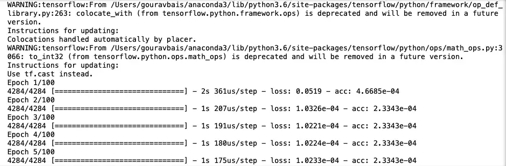
Once you execute the above code, your model training will start. It should look something like this:

Once the model is ready, you’ll need to test it on the test set to check its accuracy:

## make predictions for test set

X_test = X_test.reshape(500,1,1)

y_pred = model.predict(X_test)

## visualise results

plt.plot(y_pred, label = 'predictions')

plt.plot(y_test, label = 'actual')

plt.legend()

The graphs displaying actual labels and predicted labels should look like this:

As you can see, the predictions are the approximation of actual values, which indicates that the model is performing well enough. Since the testing data has a lot of points, the graph appears clustered; to take a closer look at the values, you can visualize just one hundred values as well:

## visualize results

plt.plot(y_pred[:100], label = 'predictions')

plt.plot(y_test[:100], label = 'actual')

plt.legend()

The simplified plot showing only one hundred actual and predicted values would be something like this:

Now, your time series forecasting model is ready, and you can use it to make predictions for upcoming dates. The code notebook for the full project can be found here.

Conclusion

In this tutorial, you learned how to do time series forecasting using deep learning framework, TensorFlow, and QuestDB. As more and more electronic and mechanical devices are becoming smart nowadays, handling them manually is ceasing to be an option. To efficiently automate the maintenance of these machines, you need to have the right tools in place to store and process machine generated data.

Traditional databases are not a good option for this, as they are more focused on processing and writing data in transactions. Time series databases, on the other hand, are specially designed for storing observations at different time intervals. They also provide features and tools to help processing time series, as you have seen in this tutorial.

If you like this content, we'd love to know your thoughts! Feel free to get started on GitHub and come say hello in our Slack Community.

Additional Resources

What is Time-Series Data?